In
analytic geometry
In classical mathematics, analytic geometry, also known as coordinate geometry or Cartesian geometry, is the study of geometry using a coordinate system. This contrasts with synthetic geometry.
Analytic geometry is used in physics and engineerin ...
, an asymptote () of a
curve
In mathematics, a curve (also called a curved line in older texts) is an object similar to a line (geometry), line, but that does not have to be Linearity, straight.
Intuitively, a curve may be thought of as the trace left by a moving point (ge ...
is a line such that the distance between the curve and the line approaches zero as one or both of the ''x'' or ''y'' coordinates
tends to infinity. In
projective geometry and related contexts, an asymptote of a curve is a line which is
tangent to the curve at a
point at infinity.
The word asymptote is derived from the
Greek ἀσύμπτωτος (''asumptōtos'') which means "not falling together", from ἀ
priv. + σύν "together" + πτωτ-ός "fallen". The term was introduced by
Apollonius of Perga
Apollonius of Perga ( grc-gre, Ἀπολλώνιος ὁ Περγαῖος, Apollṓnios ho Pergaîos; la, Apollonius Pergaeus; ) was an Ancient Greek geometer and astronomer known for his work on conic sections. Beginning from the contribution ...
in his work on
conic sections
In mathematics, a conic section, quadratic curve or conic is a curve obtained as the intersection of the surface of a cone with a plane. The three types of conic section are the hyperbola, the parabola, and the ellipse; the circle is a special ...
, but in contrast to its modern meaning, he used it to mean any line that does not intersect the given curve.
There are three kinds of asymptotes: ''horizontal'', ''vertical'' and ''oblique''. For curves given by the
graph of a
function , horizontal asymptotes are horizontal lines that the graph of the function approaches as ''x'' tends to Vertical asymptotes are vertical lines near which the function grows without bound. An oblique asymptote has a slope that is non-zero but finite, such that the graph of the function approaches it as ''x'' tends to
More generally, one curve is a ''curvilinear asymptote'' of another (as opposed to a ''linear asymptote'') if the distance between the two curves tends to zero as they tend to infinity, although the term ''asymptote'' by itself is usually reserved for linear asymptotes.
Asymptotes convey information about the behavior of curves ''in the large'', and determining the asymptotes of a function is an important step in sketching its graph. The study of asymptotes of functions, construed in a broad sense, forms a part of the subject of
asymptotic analysis
In mathematical analysis, asymptotic analysis, also known as asymptotics, is a method of describing limiting behavior.
As an illustration, suppose that we are interested in the properties of a function as becomes very large. If , then as beco ...
.
Introduction

The idea that a curve may come arbitrarily close to a line without actually becoming the same may seem to counter everyday experience. The representations of a line and a curve as marks on a piece of paper or as pixels on a computer screen have a positive width. So if they were to be extended far enough they would seem to merge, at least as far as the eye could discern. But these are physical representations of the corresponding mathematical entities; the line and the curve are idealized concepts whose width is 0 (see
Line
Line most often refers to:
* Line (geometry), object with zero thickness and curvature that stretches to infinity
* Telephone line, a single-user circuit on a telephone communication system
Line, lines, The Line, or LINE may also refer to:
Arts ...
). Therefore, the understanding of the idea of an asymptote requires an effort of reason rather than experience.
Consider the graph of the function
shown in this section. The coordinates of the points on the curve are of the form
where x is a number other than 0. For example, the graph contains the points (1, 1), (2, 0.5), (5, 0.2), (10, 0.1), ... As the values of
become larger and larger, say 100, 1,000, 10,000 ..., putting them far to the right of the illustration, the corresponding values of
, .01, .001, .0001, ..., become infinitesimal relative to the scale shown. But no matter how large
becomes, its reciprocal
is never 0, so the curve never actually touches the ''x''-axis. Similarly, as the values of
become smaller and smaller, say .01, .001, .0001, ..., making them infinitesimal relative to the scale shown, the corresponding values of
, 100, 1,000, 10,000 ..., become larger and larger. So the curve extends farther and farther upward as it comes closer and closer to the ''y''-axis. Thus, both the ''x'' and ''y''-axis are asymptotes of the curve. These ideas are part of the basis of concept of a
limit
Limit or Limits may refer to:
Arts and media
* ''Limit'' (manga), a manga by Keiko Suenobu
* ''Limit'' (film), a South Korean film
* Limit (music), a way to characterize harmony
* "Limit" (song), a 2016 single by Luna Sea
* "Limits", a 2019 ...
in mathematics, and this connection is explained more fully below.
Asymptotes of functions
The asymptotes most commonly encountered in the study of
calculus are of curves of the form . These can be computed using
limits and classified into ''horizontal'', ''vertical'' and ''oblique'' asymptotes depending on their orientation. Horizontal asymptotes are horizontal lines that the graph of the function approaches as ''x'' tends to +∞ or −∞. As the name indicates they are parallel to the ''x''-axis. Vertical asymptotes are vertical lines (perpendicular to the ''x''-axis) near which the function grows without bound. Oblique asymptotes are diagonal lines such that the difference between the curve and the line approaches 0 as ''x'' tends to +∞ or −∞.
Vertical asymptotes
The line ''x'' = ''a'' is a ''vertical asymptote'' of the graph of the function if at least one of the following statements is true:
#
#
where
is the limit as ''x'' approaches the value ''a'' from the left (from lesser values), and
is the limit as ''x'' approaches ''a'' from the right.
For example, if ƒ(''x'') = ''x''/(''x''–1), the numerator approaches 1 and the denominator approaches 0 as ''x'' approaches 1. So
:
:
and the curve has a vertical asymptote ''x'' = 1.
The function ''ƒ''(''x'') may or may not be defined at ''a'', and its precise value at the point ''x'' = ''a'' does not affect the asymptote. For example, for the function
:
has a limit of +∞ as , ''ƒ''(''x'') has the vertical asymptote , even though ''ƒ''(0) = 5. The graph of this function does intersect the vertical asymptote once, at (0, 5). It is impossible for the graph of a function to intersect a vertical asymptote (or
a vertical line in general) in more than one point. Moreover, if a function is
continuous at each point where it is defined, it is impossible that its graph does intersect any vertical asymptote.
A common example of a vertical asymptote is the case of a rational function at a point x such that the denominator is zero and the numerator is non-zero.
If a function has a vertical asymptote, then it isn't necessarily true that the derivative of the function has a vertical asymptote at the same place. An example is
:
at
.
This function has a vertical asymptote at
because
:
and
:
.
The derivative of
is the function
:
.
For the sequence of points
:
for
that approaches
both from the left and from the right, the values
are constantly
. Therefore, both
one-sided limits of
at
can be neither
nor
. Hence
doesn't have a vertical asymptote at
.
Horizontal asymptotes

''Horizontal asymptotes'' are horizontal lines that the graph of the function approaches as . The horizontal line ''y'' = ''c'' is a horizontal asymptote of the function ''y'' = ''ƒ''(''x'') if
:
or
.
In the first case, ''ƒ''(''x'') has ''y'' = ''c'' as asymptote when ''x'' tends to , and in the second ''ƒ''(''x'') has ''y'' = ''c'' as an asymptote as ''x'' tends to .
For example, the
arctangent
In mathematics, the inverse trigonometric functions (occasionally also called arcus functions, antitrigonometric functions or cyclometric functions) are the inverse functions of the trigonometric functions (with suitably restricted domains). Spec ...
function satisfies
:
and
So the line is a horizontal asymptote for the arctangent when ''x'' tends to , and is a horizontal asymptote for the arctangent when ''x'' tends to .
Functions may lack horizontal asymptotes on either or both sides, or may have one horizontal asymptote that is the same in both directions. For example, the function has a horizontal asymptote at ''y'' = 0 when ''x'' tends both to and because, respectively,
:
Other common functions that have one or two horizontal asymptotes include (that has an
hyperbola as it graph), the
Gaussian function the
error function
In mathematics, the error function (also called the Gauss error function), often denoted by , is a complex function of a complex variable defined as:
:\operatorname z = \frac\int_0^z e^\,\mathrm dt.
This integral is a special (non-elementary ...
, and the
logistic function
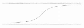
A logistic function or logistic curve is a common S-shaped curve (sigmoid curve) with equation
f(x) = \frac,
where
For values of x in the domain of real numbers from -\infty to +\infty, the S-curve shown on the right is obtained, with the ...
.
Oblique asymptotes

When a linear asymptote is not parallel to the ''x''- or ''y''-axis, it is called an ''oblique asymptote'' or ''slant asymptote''. A function ''ƒ''(''x'') is asymptotic to the straight line (''m'' ≠ 0) if
:
In the first case the line is an oblique asymptote of ''ƒ''(''x'') when ''x'' tends to +∞, and in the second case the line is an oblique asymptote of ''ƒ''(''x'') when ''x'' tends to −∞.
An example is ''ƒ''(''x'') = ''x'' + 1/''x'', which has the oblique asymptote ''y'' = ''x'' (that is ''m'' = 1, ''n'' = 0) as seen in the limits
:
 In
In  The idea that a curve may come arbitrarily close to a line without actually becoming the same may seem to counter everyday experience. The representations of a line and a curve as marks on a piece of paper or as pixels on a computer screen have a positive width. So if they were to be extended far enough they would seem to merge, at least as far as the eye could discern. But these are physical representations of the corresponding mathematical entities; the line and the curve are idealized concepts whose width is 0 (see
  ''Horizontal asymptotes'' are horizontal lines that the graph of the function approaches as . The horizontal line ''y'' = ''c'' is a horizontal asymptote of the function ''y'' = ''ƒ''(''x'') if
: or .
In the first case, ''ƒ''(''x'') has ''y'' = ''c'' as asymptote when ''x'' tends to , and in the second ''ƒ''(''x'') has ''y'' = ''c'' as an asymptote as ''x'' tends to .
For example, the
  When a linear asymptote is not parallel to the ''x''- or ''y''-axis, it is called an ''oblique asymptote'' or ''slant asymptote''. A function ''ƒ''(''x'') is asymptotic to the straight line (''m'' ≠ 0) if
:
In the first case the line is an oblique asymptote of ''ƒ''(''x'') when ''x'' tends to +∞, and in the second case the line is an oblique asymptote of ''ƒ''(''x'') when ''x'' tends to −∞.
An example is ''ƒ''(''x'') = ''x'' + 1/''x'', which has the oblique asymptote ''y'' = ''x'' (that is ''m'' = 1, ''n'' = 0) as seen in the limits
:
 ''Horizontal asymptotes'' are horizontal lines that the graph of the function approaches as . The horizontal line ''y'' = ''c'' is a horizontal asymptote of the function ''y'' = ''ƒ''(''x'') if
: or .
In the first case, ''ƒ''(''x'') has ''y'' = ''c'' as asymptote when ''x'' tends to , and in the second ''ƒ''(''x'') has ''y'' = ''c'' as an asymptote as ''x'' tends to .
For example, the